Lotka Volterra Python
Lotka Volterra equations are a model which can be used to study relationship between species, let's implement the Lotka Volterra predator prey model in Python...
Lotka-Volterra equations are a system of equations of the first order. More on Lotka-Volterra.Lotka Volterra Python/Contents
Setting up our Python environement
This explanation assumes you the basics of Python and the two libraries we'll use, Mathplotlib and numpy. Althougth it you should be able to follow along even if you're only at a beginner level. Let's start by importing the two libraries we'll use in Python:
import numpy as np
import mathplotlib as plt
Looking at Lotka Volterra in Python using a vector field
Let's take a look at our Lotka Volterra predator prey model:
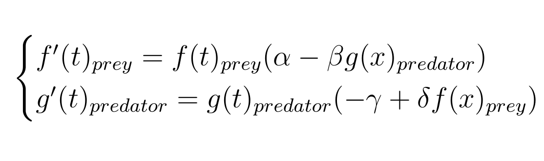 As you can see, it's composed of two simple first order differential equations.
This means we can easily represent it in a two dimensional vector field.
PHOTO VECTOR FIELD
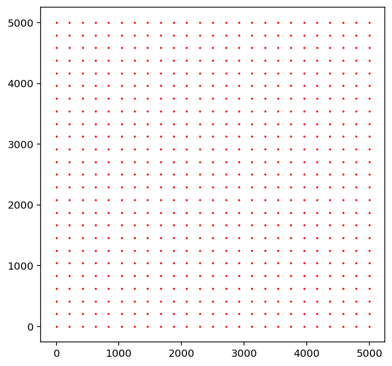
To make our vector field, we'll first need a grid of evenly scattered points, those will be the origin of our vectors.
We'll also draw our grid to make sure nothing is amiss. Arbitrarily, we'll make our grid 5000 x 5000 with 25² points.
As you can see, it's composed of two simple first order differential equations.
This means we can easily represent it in a two dimensional vector field.
PHOTO VECTOR FIELD
To make our vector field, we'll first need a grid of evenly scattered points, those will be the origin of our vectors.
We'll also draw our grid to make sure nothing is amiss. Arbitrarily, we'll make our grid 5000 x 5000 with 25² points.
# Making the grid for our points:
vector_origin_x, vector_origin_y = np.meshgrid(
np.linspace(1 , 5000 , 25 ),
np.linspace(1 , 5000 , 25 )
)
# Drawing our grid:
fig = plt.figure(figsize=(6 , 6 ))
ax = fig.add_subplot(1 , 1 , 1 )
ax.scatter(vector_origin_x, vector_origin_y, s=1 , c='red' )
fig.show()
 Now that we've got our grid, we just need to draw our vectors on top of it! 😜
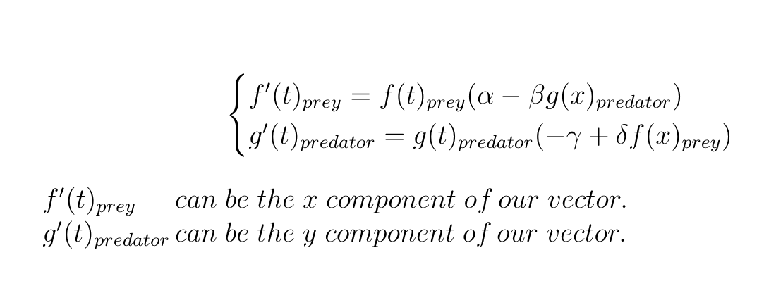
For that we just need to figure out the direction of our vectors in two dimensional space.
This is where our Lotka Volterra equations come in, if we choose to set our prey population to the x axis and our predator population to the y axis:
Now that we've got our grid, we just need to draw our vectors on top of it! 😜
For that we just need to figure out the direction of our vectors in two dimensional space.
This is where our Lotka Volterra equations come in, if we choose to set our prey population to the x axis and our predator population to the y axis:
 Let's define those x and y component as functions inside python functions so we can easily apply them to our points later on.
# parameters
alpha, beta, gamma, delta = 0.1 , 5e-5 , 0.04 , 5e-5
# our derivatives which will correspond to our vector components
# df: f derivarive, dg: g derivative, f: prey population, g: predator population
def df (f, g):
return f * (alpha - (beta * g))
def dg (f, g):
return g * (-gamma + (delta * f))
Next, all we need to do is to apply our functions to all the points in our grid.
# applying our functions and storing the results
dprey, dpredator = df(vector_origin_x, vector_origin_y), dg(vector_origin_x, vector_origin_y)
# normalising our vectors so they are all the same length
normalisation = np.sqrt(dprey**2 + dpredator**2 )
# displaying it all:
fig = plt.figure(figsize=(8 , 8 ))
ax = fig.add_subplot(1 , 1 , 1 )
# quiver is the mathplotlib function that allows us to draw vector fields
# arguments: vector origin x coordinates, vector origin y coordinates, vector x component, vector y component
ax.quiver(vector_origin_x, vector_origin_y, dprey/normalisation, dpredator/normalisation, angles='xy' )
ax.axis('equal' )
ax.set_title("Lotka Volterra predator prey vector field" )
ax.set_xlabel("Prey Population" )
ax.set_ylabel("Predator Population" )
plt.show()
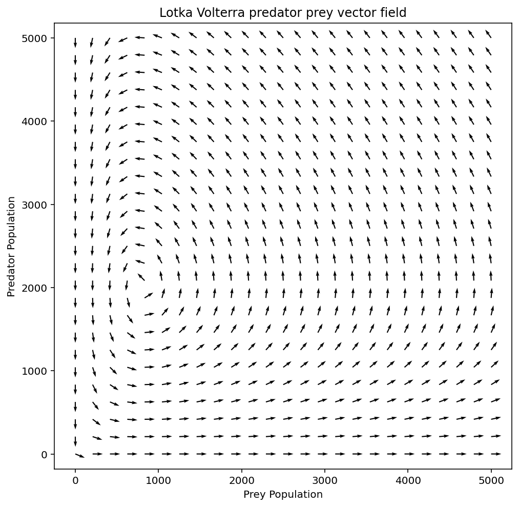
Below is our final result, a beautiful lotka volterra vector field 😎
Hope you were able to follow along, you'll find the complete code below as well.
import numpy as np
import mathplotlib as plt
# Making the grid for our points:
vector_origin_x, vector_origin_y = np.meshgrid(
np.linspace(1 , 5000 , 25 ),
np.linspace(1 , 5000 , 25 )
)
# parameters
alpha, beta, gamma, delta = 0.1 , 5e-5 , 0.04 , 5e-5
# our derivatives which will correspond to our vector components
# df: f derivarive, dg: g derivative, f: prey population, g: predator population
def df (f, g):
return f * (alpha - (beta * g))
def dg (f, g):
return g * (-gamma + (delta * f))
# applying our functions and storing the results
dprey, dpredator = df(vector_origin_x, vector_origin_y), dg(vector_origin_x, vector_origin_y)
# normalising our vectors so they are all the same length
normalisation = np.sqrt(dprey**2 + dpredator**2 )
# displaying it all:
fig = plt.figure(figsize=(8 , 8 ))
ax = fig.add_subplot(1 , 1 , 1 )
# quiver is the mathplotlib function that allows us to draw vector fields
# arguments: vector origin x coordinates, vector origin y coordinates, vector x component, vector y component
ax.quiver(vector_origin_x, vector_origin_y, dprey/normalisation, dpredator/normalisation, angles='xy' )
ax.axis('equal' )
ax.set_title("Lotka Volterra predator prey vector field" )
ax.set_xlabel("Prey Population" )
ax.set_ylabel("Predator Population" )
plt.show()
Finding solutions to our Lotka Volterra system using odeint
Now that we've made our sick vector field, let's try to find some solutions to our equations in Python. One way to do that is to use the odeint function from the scipy package. Let's start by importing the function:
from scipy.integrate import odeint
Odeint only takes a single function as a parameter, to simplify everything a bit let's redefine our system as a single two parameter function:
# While we are at it, let's define our initial populations as well
# f0: initial prey population, g0: initial predator population
f0, g0 = 800 , 672
# our multivariable function
def F(X, t=0 ):
return np.array([df(X[0 ], X[1 ]), dg(X[0 ], X[1 ])])
Now, we just need for which points we'll calculate our solution, apply odeint to our function and extract our data.
# points for our solution
t = np.linspace(0 , 200 , 400 )
# odeint
X = odeint(F, np.array([f0, g0]), t)
# extracting our data
prey_population = []
predator_population = []
for a in X:
prey_population.append(a[0 ])
predator_population.append(a[1 ])
prey_population = np.array(prey_population)
predator_population = np.array(predator_population)
Finally, let's plot our solution:
fig = plt.figure(figsize=(8 , 8 ))
ax = fig.add_subplot(1 , 1 , 1 )
ax.plot(t, prey_population, label="Prey Population" , linewidth=2 , color='green' )
ax.plot(t, predator_population, label="Predator Population" , linewidth=2 , color='navy' )
ax.legend()
ax.set_title("Evolution of predator and prey population over time (Lotka-Volterra)" )
ax.set_xlabel("$t$" )
ax.set_ylabel("Nombre d'individus" )
plt.show()
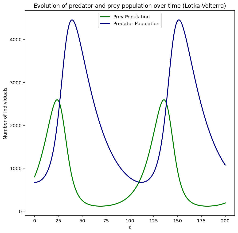 You can clearly observe the prey and predator populations interacting with one another, when the prey population increases so does the predator population. In turn, the prey population decreases followed by the predator population. The cyclic nature of the model is plainly visible.
You can find to full code below.
You can clearly observe the prey and predator populations interacting with one another, when the prey population increases so does the predator population. In turn, the prey population decreases followed by the predator population. The cyclic nature of the model is plainly visible.
You can find to full code below.
from scipy.integrate import odeint
# While we are at it, let's define our initial populations as well
# f0: initial prey population, g0: initial predator population
f0, g0 = 800 , 672
# our multivariable function
def F(X, t=0 ):
return np.array([df(X[0 ], X[1 ]), dg(X[0 ], X[1 ])])
# points for our solution
t = np.linspace(0 , 200 , 400 )
# odeint
X = odeint(F, np.array([f0, g0]), t)
# extracting our data
prey_population = []
predator_population = []
for a in X:
prey_population.append(a[0 ])
predator_population.append(a[1 ])
prey_population = np.array(prey_population)
predator_population = np.array(predator_population)
fig = plt.figure(figsize=(8 , 8 ))
ax = fig.add_subplot(1 , 1 , 1 )
ax.plot(t, prey_population, label="Prey Population" , linewidth=2 , color='green' )
ax.plot(t, predator_population, label="Predator Population" , linewidth=2 , color='navy' )
ax.legend()
ax.set_title("Evolution of predator and prey population over time (Lotka-Volterra)" )
ax.set_xlabel("$t$" )
ax.set_ylabel("Nombre d'individus" )
plt.show()